
To understand the optimization, one has to understand the digital lock-ins of the NanoScope V Controller. The vector diagram below illustrates a number of properties of the digital lock-ins, without going into the details of the actual lock-in implementation. The digital lock-in implementation phase angle varies between –180 and +180 degrees, not 0 to 360 degrees, and the raw outputs of the lock-ins are the InPhase and Quadrature values.
Figure 1: Vector diagram of E field and Sample oscillation vectors for zero drive phase
Let DE1 be the initial drive phase vector. Suppose that this corresponds to a PR drive phase of zero degrees, which corresponds to the measurement performed in PFM Optimized Vertical Domains Operation. When the drive phase is set to zero, certain domains of the PPLN samples expand and contract in-phase with the applied electric field, and others expand and contract 180 degrees out-of-phase with the applied electric field. The measured phase difference in the image results from these domains expanding and contracting 180 degrees out of phase with the applied electric field. Let such vector be represented by DS1. The suffixes E and S correspond to the electric field and the sample.
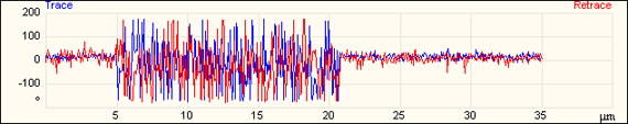
When the drive phase is zero degrees the measured (and displayed) sample vector is actually an average of a number of vectors, denoted by DS1' and DS1'' and so on. These vectors lie in the second and the third quadrant with the measured phase value being very close to the ±180 degree line. Thus the measured phase angle difference oscillates between values of –180 degrees (corresponding to vector DS1") and +180 degrees (corresponding to vector DS1'). Hence the phase contrast is not optimal. This is illustrated by a scope trace. It is also easy to imagine how the phase contrast is zero at certain points mainly due to averaging.
Next consider the case where the drive phase is 90 degrees. DE2 is the new drive phase vector. The sample vector now rotates to DS2. When the drive phase is 90 degrees, the measured (and displayed) sample vector is again an average of a number of vectors, denoted by DS2' and DS2", and so on. These vectors now lie in the third and the fourth quadrant with the measured phase value being very close to the –90 degree line. Thus the measured phase angle difference does not oscillate as it did for values of –180 degrees (corresponding to vector DS1" of Figure 1) and +180 degrees (corresponding to vector DS1' of Figure 1). This results in optimal phase contrast.

Figure 2: Vector diagram of E field and Sample oscillation vectors for 90° drive phase
Optimal phase contrast is illustrated by an actual scope trace.
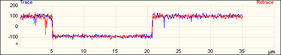
Figure 3: Scope trace of the phase channel with drive phase = 90 degrees
In this case, the averaging works to the advantage of the user. The measured phase difference between the two domains is very close to the ideal 180 degrees.
| www.bruker.com | Bruker Corporation |
| www.brukerafmprobes.com | 112 Robin Hill Rd. |
| nanoscaleworld.bruker-axs.com/nanoscaleworld/ | Santa Barbara, CA 93117 |
| Customer Support: (800) 873-9750 | |
| Copyright 2010, 2011. All Rights Reserved. |
 Related Topics